Solving complicated problems with decision tree
A decision tree is a graphical representation of possible solutions to a problem based on given conditions. It is called a tree because diagrammatically it starts with a single box (target variable) and ends up in numerous branches and roots (numerous solutions). It is a type of supervised learning algorithm that has target variables and in order to select solutions, it creates classifications. Based on classifications, however, it is applied to both categorical and continuous variables.
Using a decision tree, the population or samples can be split into two or more homogeneous sets. These homogeneous sets are constructed based on the most significant differentiator on input variables.
For example: suppose one has to buy a new mobile phone and is confused which brand to buy. So, the decision of that person depends on the amount of money he can spend. Therefore, the target variable here is ‘budget’. Further the possible solutions for buying a phone will be taken from ‘budget’.

Suppose if the buyer has less than Rs. 20,000 to spend on a mobile phone. The buyer can buy a variety of different mobiles from Companies 1 and 2, but cannot afford any mobile phone from other companies. So, representing this situation diagrammatically, a decision tree is made to classify the solutions in homogeneous groups of ‘budget’. This example is to provide a basic idea about how a decision tree works. In analytics, decision trees are applied in complex problems and the algorithm generates thousands of possible solutions for a problem.
Example of decision tree analysis
In this example, basic information of 70 patients is taken into consideration to see which of them are more prone to lung cancer. However, not more than two attributes, ‘Age’ and the habit of ‘Smoking’ has been tested against the possibility of having lung cancer.

Figure 2: Decision tree for lung cancer using R programming
The figure above shows the decision tree and explains the importance of each attribute along with the rules distinguishing between both the groups in the target variable. The rules defined by the decision tree are:
1) Rule number: 4 [Outcome=Infected cover=27 (39%) prob=0.22]

Smoking = Smoke

Age >= 25.5
This explains that there are 78% chances of the patients getting lung cancer if they smoke and are over the age of 25, according to this model.
2) Rule number: 5 [Outcome=Non-Infected cover=7 (10%) prob=0.71]

Smoking = Smoke

Age < 25.5
This rule node explains that out of all the patients there is 71% probability of patients not having lung cancer if they smoke but also are less than the age of 26.
3) Rule number: 3 [Outcome=Non-Infected cover=36 (51%) prob=0.83]

Smoking = Dont Smoke
This rule tells that if the patients don’t smoke, no matter what their age is, there is just a 17% probability of them having lung cancer. This means 83% of the total patients who don’t smoke are safe from lung cancer.
This decision tree model helped to understand the probability of patients having lung cancer based on two of the main attributes. Also, it helped to predict and identify which of the new patients are most likely to have lung cancer.
The probability of having lung cancer
Now computing the probability of having lung cancer using this decision tree. For a better understanding of it, a new simplified decision tree has been derived using the output decision tree from R.
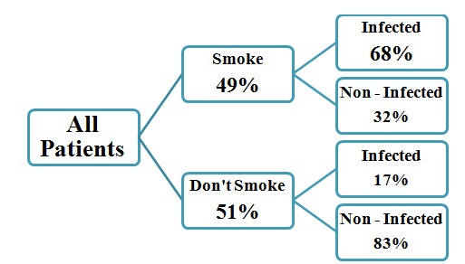
Using the decision tree in the figure above:
= probability of patients who smoke having lung cancer + probability of patients who don’t smoke having lung cancer

= [0.49 x 0.68] + [0.51 x 0.17]

= 0.33 + 0.09

=0.4199

= 41.99% chance of having lung cancer.
This is the mathematical representation of the above decision tree in Figure 3. It shows the total percentage of patients having lung cancer out of all the patients who come in. It is not very difficult to calculate the probability of an outcome using the decision tree after values are presented numerically.
Applications of decision tree analysis
- Decision trees are useful in biomedical engineering for identifying features to be used in implantable devices.
- Decision trees have been recently used to non-destructively test welding quality for semiconductor manufacturing. This helps in increasing productivity for material procurement method selection to accelerate rotogravure printing for process optimization in electrochemical machining, schedule printed circuit board assembly lines to uncover flaws in a Boeing manufacturing process and quality control.
Software supporting decision tree applications with multiple independent variables are R, SAS, MATLAB, PYTHON and SPSS.
Discuss