How to perform point forecasting in STATA?
A previous article demonstrated how to predict values for a variable that follows an autoregressive process. It showed that the first step is to identify an appropriate order of the autoregressive process. Then perform ARIMA modelling of the variable before generating the forecast. This article explains how to perform point forecasting in STATA, where one can generate forecast values even without performing ARIMA. Therefore, it is useful in any time series data.
Forecasting is an important part of time series analysis. A point forecast is a singular number which represents the estimate of the true but unknown value of a variable at a future date. The data on Gross Domestic Product (GDP), Gross Fixed Capital Formation (GFC) and Private Capital Consumption (PFC) for the same time period (1997 to 2017) as considered in the previous article is used.
Order now
Performing point forecasting in STATA
Step 1: Declare data as time series
The first step is to declare the data to be time series. For this, follow the below steps.
Stata command:

This will arrange the time series data as follows.

In the figure above, the last observation is 2017. To use point forecasting, extend the data for some more years depending on which forecast values are needed using ‘tsappend’ command.
tsappend, add(3)
tsappend, last (2020Q4) tsfmt(tq)
This command will add time period until 2020.Alternatively, use the following command.

Observations up to 2017 are ‘in-sample’ observations whereas observations after 2017 are ‘out of the sample’ observations (figure above).
Step 2: Use regression coefficients
Then use the regression coefficients with the following command.
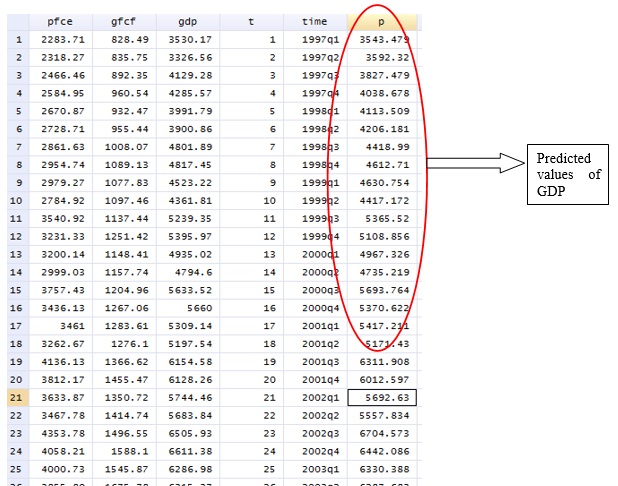
regress gdp gfcf pfceAfter the regression, use the ‘predict’ command for point forecasting, so long as the regressors are available. ‘p’ is any new variable representing GDP (since GDP is the dependent variable in the regression model). Step 3: Use the ‘predict’ command.
predict pIn-sample and out of sample data: The command ‘predict p’ will generate forecast values for in sample observations and out-of-sample observations.
To restrict the forecasting to be in‐sample (for quarterly data), use the following command.
predict p if t<=tq(2017q4)
predict yp if t>tq(2017q4)
For the out of sample (for quarterly data) prediction use the following command. This command will give forecast values of gdp, (here in p variable) in the data set (figure below).
To plot GDP and ‘p’ in graph, use the following command.
tsline gdp pThe figure below will appear.

The figure above represents the actual values and forecast values of GDP (p variable). The figure shows that there is a very slight difference actual GDP and forecast GDP values. It implies that in this case, point forecasting can effectively generate forecasted values of GDP for any time period in future.
Shortcomings of point forecasting
In point forecasting, the prediction is possible at each specific point of the data series. However, one criticism of point forecasting is that it does not provide the degree of uncertainty that is associated with the forecast. To take into account variability in forecasting, interval forecasting is applicable as an alternative to point forecasting.
I am a management graduate with specialisation in Marketing and Finance. I have over 12 years' experience in research and analysis. This includes fundamental and applied research in the domains of management and social sciences. I am well versed with academic research principles. Over the years i have developed a mastery in different types of data analysis on different applications like SPSS, Amos, and NVIVO. My expertise lies in inferring the findings and creating actionable strategies based on them.
Over the past decade I have also built a profile as a researcher on Project Guru's Knowledge Tank division. I have penned over 200 articles that have earned me 400+ citations so far. My Google Scholar profile can be accessed here.
I now consult university faculty through Faculty Development Programs (FDPs) on the latest developments in the field of research. I also guide individual researchers on how they can commercialise their inventions or research findings. Other developments im actively involved in at Project Guru include strengthening the "Publish" division as a bridge between industry and academia by bringing together experienced research persons, learners, and practitioners to collaboratively work on a common goal.
Discuss